

Social Profile of Illicit Alcohol Consumers

Abstract
This paper examines the association between social profiles and illicit alcohol consumption in Embakasi East, Nairobi, focusing on two key indicators: frequency of visits to illicit alcohol outlets and quantity consumed per session. Using a quantitative cross-sectional design, data were collected from 119 current and former consumers through structured surveys. This paper shows that males (80%), unmarried individuals (75%), and adults aged 30–39 (46%) were significantly more likely to visit illicit alcohol outlets more than five times per week. Similarly, high-volume consumption; over 4 litres per visit was most prevalent among males (30%), individuals with no formal education (55%), low-income earners earning less than KES 10,000 (50%), and the unmarried (70%). The type of illicit alcohol consumed showed no significant association with either frequency or volume. These findings offer a granular social profile of high-risk consumers and underscore the need for targeted, socially informed interventions beyond conventional regulatory approaches.
Introduction
Background
The pervasive issue of illicit alcohol addiction presents a significant public health challenge with far-reaching societal consequences, yet a comprehensive understanding of the specific social and demographic profiles of those affected remains limited. The magnitude of this problem is evidenced by studies showing a high prevalence of addiction and its association with poverty, academic failure, and other socio-economic factors. However, existing research often fails to provide an individual-level analysis of the factors driving this issue. This paper addresses this gap, and its objectives are threefold: to examine the influence of individual income, education, and family situation on the consumption of illicit alcohol; to assess the role of socio-environmental factors in predicting this behaviour; and to construct a comprehensive social profile of illicit alcohol addicts to inform more effective and targeted interventions.
Existing studies examine the demographic factors that contribute to illicit alcohol consumption (Gitatui et al., 2019; Mutisya & Justin, 2009; Kihuria, 2012; Ren et al., 2020). However, these studies rarely differentiate between factors that lead to increased consumption of illicit versus licit alcohol. Research has generally linked illicit alcohol consumption to household income (Mutisya & Justin, 2009). Some studies, though, conduct a more granular analysis, considering individual income and consumption.
Andrienko and Nemtsov (2005) demonstrated through a Tobit model that individual income significantly affects the demand for alcoholic beverages in Russia. A higher individual income is associated with a lower consumption of illicit alcohol but a higher consumption of vodka, beer, and wine. Similarly, Clements and Selvanathan (1991) found that individual income is a strong determinant of alcohol consumption in Australia. Their work classified beer and wine as necessities, while spirits were considered a luxury based on income elasticity calculations.
An individual's educational level influences the likelihood of engaging in binge drinking of illicit brews (Kihuria, 2012). Higher education is strongly associated with a decreased likelihood of consuming illicit brew, and this relationship is more pronounced at higher educational levels, such as master's or doctoral degrees. The authors suggest this correlation is linked to healthier lifestyle habits encouraged by education. Castaño and Calderon (2014) reported similar findings, observing that university students in higher levels of study, such as doctoral programmes, consume less alcohol.
Kinoti and Harper (2011) assessed high levels of illicit alcohol use in rural Kenya, specifically regional brews like Chang’aa and Busaa. Their study found that men were more likely to consume illicit alcohol than women, who generally had higher levels of employment and education. Less substance usage was typically linked to higher employment and education levels. A study in Copenhagen by Haug et al. (2009) examined alcohol consumption among adolescents, revealing an increase in consumption and weekly drunkenness between the ages of 13 and 15. The study suggested that socio-environmental factors influence adolescent alcohol choices, underscoring the importance of policy-makers in fostering healthy environments.
Kipchumba et al. (2022) investigated the drivers for the production and sale of illegal artisanal alcohol in Kakamega and Uasin-Gishu counties. The study, which included data from government administrators and illicit brew sellers, identified several contributing factors, including poverty, weak enforcement, bribery, and strong demand for the products.
The influence of family situation on alcohol consumption has received limited attention. A United States study indicated that married individuals were more likely to drink regularly than unmarried individuals (Boschuetz et al., 2020), a difference potentially linked to social behaviour. Wakeman et al. (2020) conducted a survey in a general hospital and found that men were three times more likely to drink alcohol than women, both in terms of frequency and quantity. However, the findings of Qian et al. (2018) present a different perspective, showing that married individuals and those with children are more likely to abstain from alcohol. This contrasts with earlier studies, such as Wu et al. (2008), that reported higher drinking rates among married people. Qian et al. (2018) suggested that health information about the risks of alcohol during pregnancy may influence couples planning for children. Interestingly, while those with children are more likely to abstain, those who do drink tend to be in higher income and education brackets.
GWEU Crawley (2005) explored the community and social dimensions of illicit alcohol addiction. The study estimated that 10% to 15% of the global population had succumbed to alcoholism and drug addiction. It highlighted that religious authorities often seemed unaware of the struggles of these individuals, many of whom lived in marginalised areas. The research revealed a surge in illicit alcohol addiction, urging churches to examine the factors driving this trend. Keyes and Hasin (2008) established a relationship between school performance and alcohol consumption, noting that alcohol can be both a cause and a consequence of academic failure.
From the above background it is validate to claim that illicit alcohol consumption remains a persistent public health and social challenge in Kenya, particularly within informal urban settlements. Despite widespread prevalence, there is limited empirical understanding of the specific social profiles that drive or sustain this behaviour. This gap hinders the design of targeted interventions and policy responses aimed at reducing harm and curbing illicit alcohol use. Thus, this paper attempts to research on the nexus between social profile and illicit alcohol addicts. This study is guided by the following hypotheses: 1) H1: Some social profiles are more strongly associated with higher frequency of visits to illicit alcohol consumption. 2) H2: Some social profiles are more likely to be linked with greater volumes of illicit alcohol consumption per visit.
Methods
Study Design
A quantitative cross-sectional research design was employed, integrating both descriptive and correlational approaches. The study is classified as cross-sectional because data were collected at a single point in time from a diverse sample of participants. This design is particularly effective for providing a "snapshot" of the current state of affairs regarding illicit alcohol consumption within the population. The descriptive component of the design was utilised to analyse numerical data and characterise the emerging social trends and demographic profiles of illicit alcohol consumers. Furthermore, a correlational approach was adopted to quantitatively assess the statistical association between the independent variables (such as income, education, and family situation) and the dependent variable (illicit alcohol consumption). This design enabled the identification of factors associated with increased illicit alcohol consumption, providing a basis for making predictions and generating hypotheses for future research. It is important to note that while this design can identify relationships, it does not establish cause and effect.
Population and Sample
The study population consisted of current and former illicit alcohol consumers in Embakasi East Sub-county's informal settlements, a "hidden" population due to stigma (Ellard-Gray et al., 2015). A sample size of 119 was determined using the multiplier method (Rutterford & Eldridge, 2015), with males making up 77.3% of the participants. This method estimates the population size by multiplying the number of attendees at a service or event by the inverse proportion of the population who reported attending it in a survey.
N = size of the estimated population;
x = size of the selected subgroup for which good information is available;
X = proportion of the population taking survey.
According to NACADA (2022, p.22), the estimated number of illicit alcohol users is estimated to be 57,982 in Nairobi, which represents 10.9% of total 531946 alcohol users in Kenya. Given that Embakasi East Sub-county presents 5.6% of entire Nairobi population according to 2019 Kenya population census, the proportion of 3,860.87 adults illicit alcohol consumers would be 3247(KNBS, 2019). Thus, after determining possible total population of illicit alcohol users in Embakasi East, the formula proposed in [] to identify an appropriate sample size that could guide purposive and snow-ball sample till the target is made. The steps are documented in equation [2];
Where x = 3860.87 according to Conroy (2015), for large population of less than 10,000, it is advisable to utilize a minimum ratio of more than 10% of the entire population number. Therefore, X= would be 3247.
118.6.
The determined sample size is 119; and it is therefore distributed based on different type of illicit alcohol as presented in Table 1
| Target sample | Actual sample | |
|---|---|---|
| Active consumers | 95 | 87 |
| Former consumers | 23 | 31 |
| Total | 118 | 119 |
Sampling Procedure
In this study, a two-stage cluster sampling technique was employed to address the challenges of accessing a "hidden" population of illicit alcohol consumers (Ellard-Gray et al., 2015). Given the stigma associated with this population, individuals are often reluctant to provide information, making traditional sampling frames unusable. To mitigate potential sampling bias, a subset of villages was first randomly selected from the 15 locations within Embakasi East Sub-county. The total sample size was then distributed across these chosen clusters. This method is a cost-effective design for obtaining data from a large geographical area without needing to recruit participants from every location (Wu et al., 2020). This approach differs from stratified sampling, which requires representation from all strata to reduce variance. In this case, the sampling frame consisted of the list of villages and the household size in each village. The first stage of sampling involved selecting 7 clusters (villages) out of the total 15 villages in Embakasi East Sub-county using Probability Proportion to Size (PPS). The estimator utilized the formula [3].
Where,
Where the 5% is the MOE margin of error, p is the sample proportion, and N is the population size. Z/2 is the critical value of the normal distribution at /2 (for example, for a confidence level of 95%, is 0.05 and the critical value is 1.96). The sample size formula was adjusted to account for the finite population. Through PPS sampling, it was determined that villages with more households would have a larger probability of being chosen from the sampling frame than would villages with fewer households, who would have a lesser chance. The seven (7) villages from Embakasi East Sub-county made up the study sampling frame. The sample distribution is presented in Table 2.
| Population Fraction | Sample size | |
|---|---|---|
| Donholme | 0.05 | 17 |
| Lower Savannah | 0.04 | 16 |
| Kayole North | 0.07 | 23 |
| Kwandege | 0.06 | 21 |
| Mihang’o | 0.04 | 16 |
| Embakasi Village | 0.03 | 14 |
| Utawala | 0.02 | 12 |
| Total | 119 |
After determining the number of clusters in each location and the corresponding sample size in each village, the final respondents were randomly selected from the list of villages. After establishing the sample, the researcher conducted data collection across the sub location in Embakasi East Sub County using purposive sampling and snowball where the initial contact was asked to refer any potential sample candidate given there is a high likelihood of social circle connection till the target sample size is obtained. Purposive sampling and snowball sampling procedure is the most appropriate for unknown and hidden population in quantitative research studies.
The two sample selection technique only give chance to a section of qualified population candidates that meets the purpose of the study. Equally, snowballing sampling gives chance for the first sample contact to refer the researcher to other potential sample candidates till the required sample size is obtained. (Ellard-Gray et al., 2015). This helps to address integrity and quality emanating from the data. The most appropriate sample size for any hidden population can be exhaustive as fortune would allow based on data collection timeline Therefore, such sampling method does not allow scientific calculation of sample size. Though, a study can develop a scientific formula to determine possible strategy for getting samples as maintained by Mugenda and Mugenda, (2003).
After determining the sample size for each location, the researcher embarked on the selection procedure. In this case, a non-probabilistic convenience sampling, including purposive and snowball sampling techniques, was used to recruit respondents. This approach was considered appropriate for accessing a hidden population where individuals might be reluctant to participate or reveal others (Ellard-Gray et al., 2015).
Instrument
For field data collection a questionnaire was used designed to capture social profile, gathering data on key variables such as individual income, educational level, marital status, and other relevant socio-demographic factors. The questionnaire comprised a mix of closed, open, and semi-open questions to collect both quantitative and qualitative data. A pilot study was conducted to pre-test the instrument and enhance its validity and reliability. Validity was rigorously assessed using confirmatory factor analysis, with the model's appropriateness evaluated by Chi-square, Comparative Fit Index (CFI), and Tucker-Lewis Index (TLI) tests (Bezuidenhout, 2018). Reliability of the responses was measured using simple and weighted Kappa methods and the Intraclass Correlation Coefficient (ICC), with an acceptable threshold of 0.5 (de-Felício et al., 2010).
Data Collection Procedure
Data were collected physically at the study site among the sampled villages and population in Embakasi East. The field survey method was used, as it allows for large-scale quantitative data collection while maintaining respondent anonymity and a high degree of answer reliability (Dawadi et al., Giri, 2021; Mugenda & Mugenda, 2003). Respondents completed the semi-structured questionnaire with guidance from the researcher.
Data Analysis
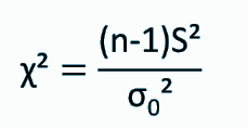
Chi-square measure of associations were completed in SPSS. The independent variables indicators included social profiles including age, gender, education level, and monthly income. The dependent variable comprised frequency visit to an illicit alcohol outlet, which was captured on a 5-Likert Scale and quantity consumed as appropriate indicator for addiction levels. Thus, a battery of Chi-square measure of association tests were completed on each socio characteristic of the illicit brew consumer. The results are provided in cross-tabulation tables along with chi-square (X2) values, Phi-values, and p-values. First, the demographic characteristics were calculated with frequency of visits to illicit alcohol outlets. Equation 4 show the chi-sure measure of association
[4]
Phi (φ) effect size
| φ = √( | χ2 | ) |
|---|---|---|
| n |
The chi-square association test inspects if the sample variance (σ2) is different from the expected value (σ02). The test also aims to test if the assumed variance (σ20) is statistically correct, based on a sample variance S2 (Govaert & Nadif, 2018). The sample size is (n).
Findings
Descriptive Findings
| Variable | Category | Frequency (%) |
|---|---|---|
| Main outlets for illicit alcohol sales | Rented houses (Homemade Moonshine) | 41 |
| Local bars/clubs (Decontaminated ethanol) | 41 | |
| Local bars/clubs (Counterfeited legal alcohol) | 30 | |
| Structure of illicit alcohol outlets | Independently (Homemade Moonshine) | 53 |
| Organised group (Decontaminated ethanol) | 34 | |
| Organised group (Counterfeited legal alcohol) | 41 | |
| Information on location of illicit alcohol sales | Social media platform | 37 |
| Awareness of seller/producer location | 33 |
Data in Table 3 indicates that rented houses and local bars/clubs are the primary outlets for illicit alcohol sales, each accounting for 41% of reported cases. Sales of counterfeited legal alcohol are slightly less common at 30%. Most homemade moonshine operations are run independently (53%), while decontaminated ethanol and counterfeit alcohol are more often distributed by organised groups. Social media (37%) and local knowledge of sellers/producers (33%) are key sources of information on these illicit activities.
Empirical Findings
| Frequency of visits at an illicit alcohol outlet (s) | |||||
|---|---|---|---|---|---|
| 1 | 2 | 3 | 4 | > 5 | |
| Less than 29 years | 67% | 50% | 40% | 39% | 36% |
| 30- 39 years | 0% | 0% | 30% | 21% | 46% |
| 40-49 years | 0% | 50% | 30% | 26% | 11% |
| 50 and above years | 0% | 0% | 0% | 10% | 7% |
| P-Value (<0.005) | 0.000 | ||||
| X2 | 60.6 | ||||
| Phi | 0.714 |
A chi-square measure of association in table 4 found statistically significant association between age of illicit consumer and frequency of visits to an illicit alcohol outlet (p=0.000, X2=60.6). Ages less than 49 years tend to visit illicit alcohols outlet more than 5 times a week as compared to their counterparts that are more than 50 years of age. Age 30- 39 years shows that at least 46% visit illicit alcohol joints more than 5 times as opposed to 7% of those aged more than 50years. The Phi value indicated a strong association of 0.714 between age and frequency visits to illicit alcohol outlet.
| Frequency of visits at an illicit alcohol outlet (s) | |||||
|---|---|---|---|---|---|
| 1 | 2 | 3 | 4 | > 5 | |
| Female | 0% | 50% | 50% | 28% | 21% |
| Male | 67% | 50% | 50% | 72% | 80% |
| P-Value (<0.005) | 0.000 | ||||
| X2 | 44.69 | ||||
| Phi | 0.613 |
A chi-square measure of association test in table 5 shows statistically significant association between gender and frequency of visits to an illicit alcohol outlet (p=0.000, X2=44.69). 80% of males visited illicit alcohols outlet more than 5 times a week as compared to only 21% of females. The phi=0.613 implies a strong association between gender and number of weekly visit to an illicit alcohol joint.
| Frequency of visits at an illicit alcohol outlet(s) | |||||
|---|---|---|---|---|---|
| 1 | 2 | 3 | 4 | > 5 | |
| Married | 35% | 45% | 48% | 30% | 25% |
| Unmarried | 65% | 55% | 52% | 70% | 75% |
| P-Value (<0.005) | 0.000 | ||||
| X² | 39.82 | ||||
| Phi | 0.587 |
A chi-square measure of association test in Table 6 shows a statistically significant association between marital status and frequency of visits to an illicit alcohol outlet (p=0.000, X²=39.82). 75% of unmarried individuals reported visiting illicit alcohol outlets more than 5 times a week, compared to only 25% of married individuals. The phi coefficient of 0.587 indicates a strong association between marital status and the frequency of visits. This suggests that unmarried individuals are more likely to frequent illicit alcohol joints than their married counterparts.
| Frequency of visits at an illicit alcohol outlet (s) | |||||
|---|---|---|---|---|---|
| 1 | 2 | 3 | 4 | > 5 | |
| decontaminated ethanol intended for industrial use/makeshifts | 5% | 30% | 45% | 5% | 15% |
| Homemade illicit brew/Moonshining (Chang’aa, kumi-kumi, busaa, Kaanga etc.) | 67% | 25% | 10% | 23% | 21% |
| Counterfeited legal alcohol (packaged in branded bottles without KEBS quality mark) | 0% | 25% | 0% | 18% | 18% |
| P-Value (>0.005) | 0.022 | ||||
| X2 | 19.93 | ||||
| Phi | 0.148 |
As presented in Table 7, consumers of homemade illicit brew have more visits to alcohol outlets than other groups. For instance, 21% visit the outlet for more than five times a week. Though, the chi-square measure of association test did not find any statistically significant association between form of illicit alcohol and frequency visits to the illicit alcohol outlet (P-Value =0.022, X2=19.93).The p-value is greater than significance level of 0.05. Thus, a lower Phi value of 0.148 was obtained meaning weak association between type of illicit alcohol and frequency of visits.
is supported by empirical evidence. Statistically significant associations were observed across age (Table 4), gender (Table 5), and marital status (Table 6), with younger, male, and unmarried individuals demonstrating higher visitation frequencies. For instance, 80% of males and 75% of unmarried individuals reported visiting illicit alcohol outlets more than five times weekly. However, no significant relationship was found between the form of illicit alcohol consumed and frequency of visits (Table 7), suggesting that behavioural patterns are more closely shaped by individual social attributes than by the type of alcohol accessed.
The second tier of Chi-square measure of association test was completed on the same social profiles with the second indicator of dependent variable (quantity consumed). Equally, a series of cross-tabulation tables were presented. To meet chi-square test data assumptions for dependent variable, the researcher recoded the quantity consumed from its continuous numerical data type to non-numerical categorical variable.
| Quantity consumed | ||||
|---|---|---|---|---|
| 2litres - 4litres | 0.5-0.9Litres | Less than half a litre | > 4 litres | |
| 18- 29 years | 30% | 21% | 19% | 30% |
| 30- 39 years | 31% | 31% | 11% | 26% |
| 40-59 years | 22% | 30% | 22% | 26% |
| 50 and above years | 9% | 45% | 18% | 27% |
| Chi-Square (X2) | 59.90 | |||
| P-Value <0.005 | 0.00 | |||
| Phi | 0.478 |
A chi-square measure of association presented in table 8 shows a statistically significant association (P-Value = 0.00) between age and average quantity consumed. More youths 3% of less than 29 years tend to consumer more illicit alcohol than consumers aged above 50 years. Though the association between age and quantity consumed is moderate, at X2= 59.90, Phi=0.478).
| Quantity consumed | ||||
|---|---|---|---|---|
| 2litres - 4litres | 0.5-0.9Litres | Less than half a litre | > 4 litres | |
| Female | 26% | 19% | 32% | 23% |
| Male | 28% | 31% | 11% | 30% |
| Chi-Square (X2) | 125.26 | |||
| P-Value <0.005 | 0.00 | |||
| Phi | 0.511 |
The chi-square measure of association findings in table 9 a statistically significant association between gender and quantity of alcohol consumed, X2=125.26, P-Value = 0.00). The association is also strong since the Phi value is 0.511. The findings show that 30% of males surveyed consumed more than 4 litre of their preferred illicit alcohol beverage as opposed to 23% of female for the same quantity. Only 11% of males consumed less than half a litre per visit as compared to 32% of females for the quantity.
| Quantity consumed | ||||
|---|---|---|---|---|
| 2litres - 4litres | 0.5-0.9Litres | Less than half a litre | > 4litres | |
| Diploma | 33% | 33% | 33% | 0% |
| No formal education | 27% | 18% | 0% | 55% |
| Post-graduate | 0% | 0% | 100% | 0% |
| Post-secondary College | 29% | 54% | 17% | 0% |
| Primary | 22% | 22% | 26% | 30% |
| Secondary | 28% | 22% | 0% | 50% |
| Undergraduate | 27% | 9% | 45% | 18% |
| Chi-Square (X2) | 17.87 | |||
| P-Value <0.005 | 0.00 | |||
| Phi | 0.609 |
As presented in Chi-square test in table 10, the association between education level and quantity consumed is strong and statistically significant (Chi-Square X2=17.87, P-Value = 0.00, Phi=0.609. Respondents with no formal education (55%) could consume more than four litre of alcohol per visit similar to 50% with secondary education, and 30% with primary education. This is as opposed to only 18% of consumers with undergraduate education level. Besides, 45% of consumers with undergraduate education consumed less than half a litre of illicit alcohol per visit as opposed to 0% of consumers with no formal education.
| Quantity consumed | ||||
|---|---|---|---|---|
| 2litres - 4litres | 0.5-0.9Litres | Less than half a litre | More than 4litres | |
| 11,000-30,000 | 36.9% | 10.0% | 6.0% | 47.1% |
| 31,000-40,000 | 25.5% | 34.5% | 30.3% | 9.7% |
| 41,000-50,000 | 24.0% | 29.6% | 40.5% | 5.9% |
| Less than 10,000 | 23.9% | 11.8% | 14.3% | 50.0% |
| Chi-Square (X2) | 29.90 | |||
| P-Value <0.005 | 0.00 | |||
| Phi | 0.855 |
There is a statistically significant association between income level of illicit alcohol consumer and quantity consumed based on findings in table 11. Chi-Square X2= 29.90, P-Value < 0.005, Phi = 0.855. The Phi value shows an extremely high association. Most, 50.0% of low class income earners of less than 10,000 and 47.1% 11,000-30,000 Kenya Shillings a month could consume more than 4 litres of illicit alcohol per visit, compared to only 9.7% and 5.9% of consumers that earned 31,000-40,000 and 41,000-50,000 Kenya Shillings monthly, respectively.
| Quantity consumed (In liters) | |||||
|---|---|---|---|---|---|
| Married | 42% | 55% | 65% | 30% | 42% |
| Unmarried | 58% | 45% | 35% | 70% | 58% |
| P-Value (<0.005) | 0.000 | ||||
| X² | 36.14 | ||||
| Phi | 0.559 |
A chi-square test of association in Table 12 shows a statistically significant relationship between marital status and the quantity of illicit alcohol consumed (p=0.000, X²=34.27). 70% of unmarried individuals consumed more than 4 litres, compared to only 30% of married individuals. Lower levels of consumption (less than 0.55 litres) were reported by 65% of married individuals versus 35% of unmarried ones. The phi coefficient of 0.542 suggests a strong association between marital status and quantity of illicit alcohol intake.
| Quantity consumed (In liters) | ||||
|---|---|---|---|---|
| 2- 4 | 0.5-0.9 | <0.55 | > 4 | |
| Decontaminated ethanol intended for industrial use /makeshifts | 44.9% | 30.7% | 7.9% | 16.5% |
| Homemade illicit brew/Moonshining (Chang’aa, kumi-kumi, busaa, Kaanga etc.) | 9.9% | 52.5% | 31.5% | 6.1% |
| Counterfeited legal alcohol (packaged in branded bottles without KEBS quality mark) | 47.1% | 36.4% | 11.0% | 5.5% |
| Chi-Square (X2) | 11.60 | |||
| P-Value <0.005 | 0.06 | |||
| Phi | .204 |
As presented in Table 13, the Chi-square test found no statistically significant association betweentype of illicit brew and quantity consumed as presented in table4.16,X2= 11.60, P-Value=0.006, which is greater than 0.005, and a small Phi value of 0.204 was obtained. The percentage values across quantity consumed varies based on type of illicit alcohol without forming a linear or identical pattern. Though, a considerable proportion (16.5%) of consumers of decontaminated ethanol intended for industrial use tend to consumer more than 4litres per visit.
Discussion
Social Profiles and Frequency of Visits to Illicit Alcohol Outlets
The first hypothesis on the association between social profiles and frequency of visits to illicit alcohol outlets is supported by empirical evidence. Statistically significant associations were observed across age (Table 4), gender (Table 5), and marital status (Table 6). Younger, male, and unmarried individuals demonstrated notably higher visitation rates. For example, 80% of males and 75% of unmarried respondents reported visiting illicit alcohol outlets more than five times per week, compared to only 21% and 25% among females and married individuals, respectively.
These findings are consistent with previous research by Haug et al. (2009), who attributed increased alcohol use among youth to socio-environmental influences. However, this study extends that understanding to adults aged 30–39, revealing a sustained high engagement beyond adolescence. This highlights a policy gap in addressing problematic alcohol use in this demographic segment.
The pronounced gendered pattern mirrors findings by Wakeman et al. (2020) and Kinoti and Harper (2011), reinforcing the disproportionate exposure of males to alcohol-related harm. What this study adds is a higher level of granularity, capturing both visit frequency and consumption volume, which previous studies did not quantify. Similarly, marital status emerges as a critical factor; the findings align with Qian et al. (2018), suggesting that individuals without family or spousal responsibilities are more inclined toward habitual outlet visits.
Notably, the form of illicit alcohol consumed did not significantly influence frequency of visits (Table 7), as shown by the non-significant p-value and low Phi coefficient. This diverges from studies like Kipchumba et al. (2022), which focused on the product type as a driver of consumption. The findings here imply that behavioural patterns are more strongly shaped by personal and social attributes than by the specific type of illicit alcohol accessed.
4.2: Social Profiles and Quantity of Illicit Alcohol Consumed
The second hypothesis regarding the association between social profiles and the quantity of illicit alcohol consumed is also confirmed by the data. Statistically significant relationships were identified across age (Table 8), gender (Table 9), education level (Table 10), income (Table 11), and marital status (Table 12). Higher consumption volumes exceeding 4 litres per visit were disproportionately reported among younger individuals, males, those with no formal education, low-income earners, and the unmarried. For instance, 50% of respondents earning less than KES 10,000 and 55% of those without formal education reported consuming over 4 litres per session, indicating a strong link between social vulnerability and excessive intake.
The results further validate previous studies that link low education and income to alcohol abuse. Kihuria (2012) and Castaño and Calderon (2014) highlighted education as a protective factor, and this study confirms that association using direct quantity metrics. Respondents with higher education were significantly less likely to consume large volumes, reinforcing the preventative role of educational attainment. Also, income-related findings are in line with Andrienko and Nemtsov (2005), who associated higher individual income with lower consumption of illicit alcohol. However, this study provides a Kenyan-specific nuance, as it clearly distinguishes between licit and illicit behaviours, revealing the entrenched relationship between economic precarity and harmful consumption patterns.
As with visit frequency, the type of illicit brew consumed was not significantly associated with quantity (Table 13). While previous literature often pointed to certain types, such as Chang’aa or decontaminated ethanol, as high-risk (e.g. Kipchumba et al., 2022), this study shows that addiction severity is not necessarily determined by the form of alcohol but rather by broader structural and personal conditions.
Conclusion
Summary
This study provides strong empirical support for the two proposed hypotheses, establishing that some social profiles are significantly associated with both the frequency of visits to illicit alcohol outlets and the quantity consumed per session. The findings show that younger, male, unmarried, low-income, and less-educated individuals are disproportionately represented among high-frequency and high-volume consumers. These associations were statistically significant across multiple variables, with particularly strong effect sizes for age, gender, income, and marital status.
The evidence contributes new granularity to existing literature by operationalising illicit alcohol addiction through dual indicators frequency and volume and mapping these directly against social characteristics. This disaggregated analysis reveals the specific population segments most at risk, offering a data-driven basis for targeted public health interventions. Importantly, the study also clarifies that the type of illicit alcohol consumed does not significantly influence either frequency or quantity, challenging assumptions in prior research that certain brews inherently drive addictive behaviours. Overall, the study fills a critical gap in understanding the social profile of illicit alcohol consumers in Nairobi's informal settlements. Its findings should inform more differentiated and responsive strategies that prioritise high-risk social groups rather than relying solely on broad regulatory or enforcement-based approaches.
Limitations
While the study provides valuable insights, several limitations must be acknowledged. First, the sample size of 119, though adequate for exploratory analysis, may limit the generalisability of findings to broader populations beyond Embakasi East. Second, the hidden and stigmatised nature of illicit alcohol consumers necessitated non-probabilistic techniques (purposive and snowball sampling), which may introduce selection bias and underrepresent less socially connected individuals. Third, the study relied solely on chi-square tests to assess associations, which, while suitable for categorical data, do not account for interaction effects or control for confounding variables.Future research could address these limitations by employing larger, stratified samples across multiple urban areas, integrating mixed-method approaches, and applying multivariate models such as logistic regression to enhance explanatory power. Despite these limitations, the study maintains a high degree of internal reliability and validity. The structured data collection instrument was pre-tested and statistically validated, and the use of dual indicators for addiction (frequency and quantity) provides a robust framework for understanding patterns of illicit alcohol use. Thus, the findings remain credible and valuable for informing targeted intervention and policy design.
References
Rights and permissions

Disclaimer
All claims expressed in this article are solely those of the author and do not necessarily represent those of the publisher, editors, reviewers, or affiliated institutions. Any product, service, or claim that may be evaluated in this article is not guaranteed or endorsed by the publisher.
Publisher’s note
The publisher remains neutral with regard to jurisdictional claims.
Additional information
Data availability
Acknowledgements
Funding
Conflict of interest
Article Timeline
 Publication record
Cite this article
- Received
- August 9, 2025
- Revised
- August 26, 2025
- Accepted
- September 3, 2025
- Published
- September 14, 2025
- Version of record
- September 14, 2025
Share this article
Share the article record with colleagues and readers worldwide.
Explore research across our journalsDiscover more research

Recent Publications

Most Read

Recommended
Save this article as a bookmark
Use your browser’s secure bookmark shortcut. Both desktop options are shown below.
Press Ctrl+D
In Chrome, Edge or Firefox, choose a folder if needed, then select Done.
Press ⌘ Command+D
In Safari, Chrome or Firefox, choose the bookmark location and confirm.
Cite this article
Copy a formatted citation or download a reference file.
Cited by
Crossref citation count for this DOI.