

Abstract
Alcohol pricing is a central determinant of drinking choices in Nairobi’s informal settlements, where illicit brews dominate consumption. This study surveyed 118alcohol outlets and applied a multinomial logit model with controls for cost of living, outlet availability, and peer influence. Descriptive results show that respondents consumed on average 2.4 litters per visit; illicit alcohol accounted for 61% of total consumption. Empirical estimates reveal that a KES 10 increase in legal alcohol prices raised the probability of illicit alcohol choice by 8.7% (p < .01), while a KES 10 rise in illicit prices reduced consumption likelihood by 6.2% (p < .05). Peer influence and outlet density further amplified illicit substitution. These findings suggest that excise-driven price hikes, without strong enforcement and affordable alternatives, risk intensifying harmful illicit alcohol use.
Introduction
Background
Alcohol consumption policies across the world demonstrate that pricing instruments, particularly excise duties, are a central tool for shaping drinking behavior. Countries that coupled higher excise taxes with minimum unit pricing, advertising bans, and sales restrictions recorded significant declines in alcohol intake and related harm (Nelson & McNall, 2016). For example, tax hikes in Estonia, Latvia, Lithuania, and Poland reduced per capita consumption by about 0.9 liters between 2000 and 2020 (Horáková et al., 2020; Manthey et al., 2024). In Russia, minimum excise taxes combined with bottle-tracking systems, advertising restrictions, and tighter age controls reduced per capita consumption by 5.3 liters, and alcohol-related deaths fell by 1,600 between 2006 and 2017 (Neufeld et al., 2022). Similar outcomes were observed in Lithuania, Finland, and Scotland, where excise hikes and minimum pricing translated into lower alcohol sales, fewer hospitalizations, and reduced mortality (Tigerstedt et al., 2020; Holmes et al., 2022; Manthey et al., 2024).
At the same time, there is a significant number of cases where policy adjustments through excise duty increases have failed to control alcohol consumption. For example, the popular USA alcohol use restriction policies of the 1920s escalated cases of organized crime, bootlegging, and illegal speakeasies, leading to their repeal in 1933 after being identified as a failed social experiment (Kozul, 2020). In the former USSR, Mikhail Gorbachev’s anti-alcohol campaign based on bans, heavy taxation, and strict enforcement between 1985 and 1987 to reduce consumption saw a decline in alcohol use and alcohol-related mortality dropped, but this trend reversed rapidly backfired as bootlegging and illicit alcohol production surged, replacement of liquor with sugar-based homemade alcohol and an escalation in the cases of alcohol poisoning and deaths.
Eventually, the campaign was discontinued in 1988, and formally repealed in 1990 (Neufeld et al, 2021). Likewise, Turkey’s move to raise its special consumption tax on alcohol and enact sweeping restrictions on advertising and nighttime sales in 2010 drove pushed alcohol consumption underground leading to a significant increase in cases of alcohol smuggling, fraud, and alcohol circulation, and mass poisoning events like the 2011 Turkish Riviera tragedy (Matthee, 2023). Similarly, Moldova hiked alcohol taxes in 2010, restricted hours of alcohol sale, banned alcohol ads, and raised legal drinking age. However, cultural norms, together with weak enforcement made the policy ineffective in controlling total alcohol consumption and alcohol‐linked harm. Since 1977(Paraje et al., 2023) Pakistan successfully banned alcohol sales under Islamic law. However, this move did not succeed in eliminating alcohol use, especially among non-Muslims and elites. Instead, cases of illegal production and distribution of alcohol, and alcohol-related poisoning rose (Nayab et al., 2022).
Between 2004 and 2009, Kenya set excise on alcoholic beverages as both specific and ad valorem duties. For beer, the proof per litre rate was 60 percent for stout/porter. On the other hand the rates for Chibuku, wine and spirits were 10 percent, 40 percent and 60 percent. In 2010, the Alcoholic Drinks Control Act was enacted. The act retained the previous excise structure but introduced health and social component in the regulations. The new rules encapsulated alcohol production licensing, use age limits, promotional restrictions, and operating hours for alcohol sale joints upto around 2014. The successive Finance Acts from 2015 onwards raised excise duty sharply on beer, wine, and spirits via annual adjustments. By 2018, the excise structure was expanded to include KES 105.20/L in low alcohol beverages (≤ 6 percent ABV). The Finance Act of 2020 replaced mixed excise structures of the previous years with flat rates per litre. Under this policy, the excise rate for beer and low-strength beverages and (>6 percent ABV) was set at KES 110.62/L and KRD 253/L respectively. Inflation indexing and policy adjustments led to a modest rise in excise rates.
The Finance Act of 2022, raised the beer, wines and spirit excise rates to KES 134/L, KES 229/L and KES 335.30/L respectively. From 2023 through 2024, excise revenue especially from spirits declined significantly. The trend was attributed to a dramatic shift of consumers to illicit alcohol. Alcohol consumption volumes declined by approximately 29–35% between 2018 and 2024 as illicit alcohol consumption rose to ≥60 percent of total alcohol intake domestically in Kenya. The cases if alcohol poisoning also increased sharply, with The Nairobi Hospital reporting an increase in these cases by 38% . The Finance Bill 2024 proposed a shift of the excise duty to ABV based excise (KES 640/L for spirits), eliminating manufacturer input tax credits, and tightening filing windows, but mass anti-finance bill protests and the subsequent withdrawal in June 2024 paved the way for Tax Laws Amendment Act 2024, which, introduced and excise rate if KES 22.50 per centilitre of pure alcohol across beer, wine, spirits. The new policy also reduced the excise rate for small brewers to KES 10/cl. A 4.9 percent excise adjustments based on inflation indexing have been in place into 2025.
Though, not all pricing and restriction policies, however, achieve their intended outcomes. The U.S. Prohibition era and Gorbachev’s Soviet anti-alcohol campaign highlight how steep taxation or outright bans can push consumers into illicit markets, resulting in smuggling, bootlegging, poisoning, and ultimately policy failure (Kozul, 2020; Neufeld et al., 2021). Similar unintended effects emerged in Turkey, Moldova, and Pakistan, where sharp excise hikes or outright bans shifted demand toward unregulated supply chains, exacerbating health risks rather than reducing them (Matthee, 2023; Paraje et al., 2023; Nayab et al., 2022).
Despite extensive policy experimentation, the link between price shifts, substitution between licit and illicit alcohol, and consumption intensity remains underexplored in Nairobi’s informal settlements. Price not only determines choice of alcohol type but also interacts with availability, social circles, and cost of living pressures. Understanding these dynamics is crucial, since substitution toward illicit alcohol amplifies public health risks. This study therefore has two objectives: (i) to examine how relative price influences substitution between licit and illicit alcohol; and (ii) to analyse how price, together with contextual factors such as availability of outlets, peer influence, and income proxies, determines frequency and quantity of alcohol consumed.Accordingly, two hypotheses are tested: 1) Higher prices of licit alcohol significantly increase the probability of substitution toward illicit alcohol; 2) Price, together with social and contextual factors, significantly predicts consumption frequency and quantity in informal settlements.
Methods
Study Design
The study used a cross-sectional analytical design to analyse alcohol consumption in Nairobi's informal settlements. It collected quantitative data and analysed how price differences and contextual factors influenced alcohol consumption choices. The design included descriptive and inferential components, focusing on consumption intensity, type, and socio-economic profiles. The design was chosen for its feasibility, cost-effectiveness, and robust testing in the dynamic alcohol markets of Nairobi's informal settlements.
Population and Sample
The population consisted of current and past illicit alcohol consumers in the informal settlements of Embakasi East Sub-county. This population is considered "hidden" due to the stigmatised nature of their activities (Ellard-Gray et al., 2015; Otzen & Manterola, 2017). The sample size was determined using a multiplier method (Rutterford & Eldridge, 2015), drawing on population data from NACADA (NACADA, 2022) and the Kenya Population Census (KNBS, 2019). This process resulted in a determined sample size of 119 participants, distributed between active and former consumers. Male were the majority representing 92(77.3%).
The estimate is achieved by multiplying the number of attendees during a period by the proportional inverse of the population who said they attended during the same period when answering the survey designed for a research project, using the following formula (Rutterford & Eldridge, 2015):
N = size of the estimated population;
x = size of the selected subgroup for which good information is available;
X = proportion of the population taking survey.
According to NACADA (2022, p.22), the estimated number of illicit alcohol users is 57,982 in Nairobi, which represents 10.9% of total 531,946 alcohol users in Kenya. The Kenya Population Census of 2019 indicates that Embakasi East Sub-county presents 5.6% of entire Nairobi population. Considering this, out of the3, 860. 87 adults illicit alcohol consumers in Nairobi, Embakasi East has 3247(KNBS, 2019). Thus, after determining possible total population of illicit alcohol users in Embakasi East, the formula proposed in [] to identify an appropriate sample size that could guide purposive, where the researcher targets known drinkers in the targeted zone, followed by snow-ball sample till the target is made. The steps are documented in equation [2];
Where x = 3860.87 according to Conroy (2015), for large population of less than 10,000, it is admissible to utilize a minimum ratio of more than 10% of the entire population number. Therefore, the estimated X= is 3247.
118.6.
The determined sample size is 119; and it is therefore distributed based on different type of illicit alcohol as presented in Table 1.
| Target sample size | Obtained sample size | |
|---|---|---|
| Active consumers | 95 | 87 |
| Former consumers | 23 | 31 |
| Total | 118 | 119 |
Sampling Procedure
Sampling procedure are techniques and scientific approaches used to arrive at a certain sample size. In hidden populations, the true size is unknown, and individuals often refuse to provide information about other members of the group for fear of being stigmatised or identified, prosecuted, and sometimes abused because of their characteristics (Ellard-Gray et al., 2015). As a result, this research study seek to identify individuals belonging to these illicit alcohol consuming subgroups must be extensive and contain a number of subjects that allows for a correct estimate of sample size.
The next step involved determining the sample selection across various locations within Embakasi East Sub-county in order to prevent potential sample bias, particularly stemming from sampling frame bias. With 15 locations in Embakasi East, it was necessary to evenly distribute the total target sample size from Table 3.1 across the villages. To achieve this, a two-stage cluster sampling technique was utilized to select a subset of villages from the 15 available. According to Wu et al. (2020), this technique involves random sampling within clusters, each comprising multiple elementary units that are sampled twice. Two-stage cluster sampling is often a cost-effective design for obtaining required information without needing to recruit study participants from all villages in the study area. This method differs from stratified sampling, where all strata are represented in the sample with the aim of reducing estimator variance (Wu et al., 2020).
In this case, the sampling frame consisted of the list of villages and the household size in each village. The first stage of sampling involved selecting 7 clusters (villages) out of the total 15 villages in Embakasi East Sub-county using Probability Proportion to Size (PPS). The estimator utilized the formula [3].
Where,
Where the 5% is the MOE margin of error, p is the sample proportion, and N is the population size. Z/2 is the critical value of the normal distribution at /2 (for example, for a confidence level of 95%, is 0.05 and the critical value is 1.96). The sample size formula was adjusted to account for the finite population. By using PPS sampling, it was determined that villages with more households would have a larger probability of being chosen from the sampling frame than would villages with fewer households, who would have a lesser chance. The seven (7) villages from Embakasi East Sub-county made up the study sampling frame. The sample distribution is presented in Table 2.
| Clusters | Proportion | Sample size |
|---|---|---|
| Donholme | 0.05 | 17 |
| Lower Savannah | 0.04 | 16 |
| Kayole North | 0.07 | 23 |
| Kwandege | 0.06 | 21 |
| Mihang’o | 0.04 | 16 |
| Embakasi Village | 0.03 | 14 |
| Utawala | 0.02 | 12 |
| Total | 119 |
After determining the number of clusters in each location and the corresponding sample size in each village, the final respondents were randomly selected from the list of villages. After establishing the sample, the researcher conducted data collection across the sub location in Embakasi East Sub County using purposive sampling and snowball where the initial contact was asked to refer any potential sample candidate given there is a high likelihood of social circle connection till the target sample size is obtained. Purposive sampling and snowball sampling procedure is the most appropriate for unknown and hidden population in quantitative research studies.
The two sample selection technique only give chance to a section of qualified population candidates that meets the purpose of the study. Equally, snowballing sampling gives chance for the first sample contact to refer the researcher to other potential sample candidates till the required sample size is obtained. (Ellard-Gray et al., 2015). This helps to address integrity and quality emanating from the data. As Baker and Edwards (2017) allude, the most appropriate sample size for any hidden population can be exhaustive as fortune would allow based on data collection timeline Therefore, such sampling method does not allow scientific calculation of sample size. Though, a study can develop a scientific formula to determine possible strategy for getting samples as maintained by Mugenda and Mugenda, (2003).
After determining the sample size for each location, the researcher embarked on the selection procedure. In this case, a non-probabilistic convenience sampling, including purposive and snowball sampling techniques, was used to recruit respondents. This approach was considered appropriate for accessing a hidden population where individuals might be reluctant to participate or reveal others (Ellard-Gray et al., 2015).
Instruments
The data collection instrument was a questionnaire used for a field survey. It comprised closed, open, and semi-open questions to capture both numerical and categorical data (Mugenda & Mugenda, 2003). A pilot study was conducted to pre-test the questionnaire and improve its validity and reliability. The validity of the instrument was further assessed using confirmatory factor analysis, with the model's appropriateness evaluated using Chi-square, Comparative Fit Index, and Tucker-Lewis Index tests (Bezuidenhout, 2018). Reliability was measured for each variable's responses using simple and weighted Kappa methods and the Intraclass Correlation Coefficient, with a threshold of 0.5 (de-Felício et al., 2010).
Data Collection Procedure
Data were collected physically at the study site among the sampled villages and population in Embakasi East. The field survey method was used, as it allows for large-scale quantitative data collection while maintaining respondent anonymity and a high degree of answer reliability (Dawadi et al., Giri, 2021; Mugenda & Mugenda, 2003). Respondents completed the semi-structured questionnaire with guidance from the researcher.
Model
This study examines how relative prices of licit and illicit alcohol shape both (i) the choice of alcohol type and (ii) the intensity of consumption among residents of Nairobi’s informal settlements. The analysis is framed as a substitution problem: when the price of one category shifts relative to the other, consumers may switch types and/or adjust frequency of drinking and quantity consumed. The empirical strategy therefore separates the extensive margin (which type is chosen) from the intensive margin (how often and how much is consumed once a type is chosen). Thus, a Two-Part Logit–OLS Substitution Model of Alcohol Consumption was chosen. The choice model involves a binary logit model, a binary logistic regression, to predict the probability of choosing licit or illicit alcohol. The second stage involves a linear regression for consumption intensity, a standard OLS/GLM for continuous outcomes. This model is often called a Logit-OLS Substitution Model in economics.
For variables, Let PLdenote the respondent-reported market price of licit alcohol and PIthe price of illicit alcohol at the time/place typically purchased. To capture substitution, the core predictor is the relative price expressed as a log price ratio,
which is positive when licit alcohol is more expensive than illicit, zero at parity, and negative when licit is cheaper. (For robustness, we also computed the simple price difference ; results are reported using because elasticities are directly interpretable in logs.) The choice outcome is coded as if the respondent's main drink in the reference period is licit and if illicit. The intensity outcomes are (a) weekly frequency of alcohol-outlet visits and (b) quantity consumed per sitting (measured in standard units; skewed variables are log-transformed where appropriate). Three policy-relevant controls are included as dummies: a cost-of-living proxy ( rising sharply; otherwise), outlet availability ( "many outlets nearby"; "few"), and peer influence ( reports being influenced by friends; otherwise). To connect stated motives to behaviour, we also include attribution indicators (1 = respondent explicitly attributes recent change in drinking to that reason; 0 = otherwise). Unless stated, all models include a disturbance term with mean zero.
Stage 1: Alcohol-type choice (substitution at the extensive margin). The probability that a respondent chooses licit alcohol is modelled with a binary logit:
where collects all covariates. The coefficient captures the substitution effect of relative price: because rises when licit becomes more expensive relative to illicit, the expected sign is (higher relative licit price lowers the odds of choosing licit). Interaction terms all the relative-price effect to vary with peer pressure and outlet densitv.
A useful price-shift threshold (the "switching point") is obtained by solving for the relative price at which a respondent is indifferent between types, i.e., . Setting the logit to zero yields
Exponentiating gives the threshold price ratio:
the point at which the predicted choice probability is 50-50. Values above this ratio imply a higher predicted probability of choosing illicit, and values below imply a higher probability of choosing licit. Marginal effects are reported as , and we compute cross-price elasticities of choice: with respect to licit price, ; with respect to illicit price, .
Stage 2: Consumption intensity (own-price and residual substitution at the intensive margin). Conditional on the chosen type , we model frequency and quantity as functions of the own price of the chosen type, the relative price, and the same controls. For frequency,
An analogous specification is estimated for quantity per sitting (logged if skewed). Coefficients represent own-price effects (higher price of the chosen type reduces frequency/quantity), while captures any residual role of relative price after conditioning on type-e.g., when the other category becomes much cheaper, consumers may stretch sessions or add visits even if they have not switched types. Including the attribution dummies in this stage links stated reasons to observed intensity, and interactions (e.g., ) test whether self-identified "price-sensitive" drinkers react more strongly to price.
Price-shift steps and nonlinearity. Because substitution may be sharp around parity, we include (i) a parity indicator to distinguish regimes where illicit is cheaper, and (ii) flexible forms for (restricted cubic splines with a knot at and at empirical quartiles). This allows the logit slope to steepen near the price-shift step and fl atten at extremes without imposing linearity. For ease of presentation, we report both the flexible (spline) fit and a parsimonious linear specification.
Estimation and diagnostics. Stage-1 parameters are estimated by maximum likelihood (logit); we report odds ratios, robust (HC) standard errors, pseudo- , AIC, and classification metrics. Stage- 2 parameters are estimated by OLS with heteroskedasticity-robust standard errors; if or are count-like and overdispersed, we confirm robustness with negative binomial models. Multicollinearity is assessed via VIF; and are retained together only if VIF (otherwise replaces in sensitivity checks). Because Stage-2 outcomes are observed conditional on choice, we also estimate a control-function variant that adds the Stage-1 generalized residual to Stage-2 to check for selection; results are compared to the standard twopart estimates.
Interpretation. The Stage-1 coefficient and the derived threshold quantify when consumers switch types as prices move; Stage-2 coefficients and show how much frequency and quantity adjust with own and relative prices after a choice is made. The attribution terms connect perceived reasons to behavioral responses, while interactions reveal whether substitution is amplified by peer influence or outlet density under high cost-of-living conditions.
Results
Descriptive Statistics
Table 1 presents the descriptive statistics for the key study variables (N = 118). The average reported market price for licit alcohol was KES 160.40 per Litre (SD = 45.20), while illicit alcohol was notably cheaper, averaging KES 95.70 (SD = 30.80). The mean relative price ratio was 1.68, indicating that licit alcohol was on average 68% more expensive than illicit alternatives.
| Variable | M | SD | Min | Max |
|---|---|---|---|---|
| Price of licit alcohol (KES/litre) | 160.40 | 45.20 | 80 | 260 |
| Price of illicit alcohol (KES/litre) | 95.70 | 30.80 | 50 | 160 |
| Relative price ratio | 1.68 | 0.54 | 0.80 | 3.00 |
| Weekly frequency of visits | 3.42 | 1.85 | 0 | 8 |
| Quantity consumed per sitting (liters) | 2.34 | 0.92 | 0.5 | 4.0 |
| Cost-of-living pressure (dummy) | 0.61 | 0.49 | 0 | 1 |
| Outlet availability (dummy) | 0.53 | 0.50 | 0 | 1 |
| Peer influence (dummy) | 0.47 | 0.50 | 0 | 1 |
Note. Prices are in Kenyan Shillings (KES). Dummies coded as 1 = present, 0 = absent, (n = 118)
Respondents reported visiting alcohol outlets an average of 3.42 times per week (SD = 1.85) and consuming approximately 2.34 litres per sitting (SD = 0.92). More than half of participants reported significant cost-of-living pressures (61%), nearby outlet availability (53%), and peer influence on alcohol choice (47%).
Empirical Findings
The empirical results are presented in two parts: 1) a binary logistic regression (Table 2) was then employed to examine how relative price and other covariates predict the choice between licit and illicit alcohol. 2) an OLS regression (Table 3) was estimated to analyse consumption intensity, measured as frequency of visits to alcohol outlets and volume consumed per sitting, conditional on alcohol type.
Table 2 shows the results of the binary logistic regression to test whether relative prices and contextual factors predict the likelihood of choosing licit alcohol. The model was significant, χ²(4) = 22.84, p < .001, Nagelkerke R² = .27. Relative price ratio significantly reduced the odds of choosing licit alcohol (B = –1.42, SE = 0.51, OR = 0.24, p = .005**). Outlet availability (B = –0.92, p = .028*) and peer influence (B = –1.11, p = .014*) also significantly decreased licit alcohol choice, while cost-of-living pressures were marginal (p = .082).
| Predictor | B | SE | Wald | OR | 95% CI for OR | p |
|---|---|---|---|---|---|---|
| Relative price ratio (ρ) | –1.42 | 0.51 | 7.80 | 0.24 | [0.09, 0.66] | .005** |
| Cost-of-living (dummy) | –0.68 | 0.39 | 3.03 | 0.51 | [0.23, 1.15] | .082 |
| Outlet availability | –0.92 | 0.42 | 4.79 | 0.40 | [0.18, 0.92] | .028* |
| Peer influence | –1.11 | 0.45 | 6.05 | 0.33 | [0.13, 0.81] | .014* |
| Constant | 2.75 | 0.88 | 9.80 | 15.6 | — | .002** |
Note. OR = odds ratio. Nagelkerke R² = .27. Model χ²(4) = 22.84, p < .001.
Statistical significance is denoted by *p < .05, **p < .01, and ***p < .001.
The hypothesis that higher relative prices reduce the probability of licit alcohol consumption was supported, B = –1.42, SE = 0.51, OR = 0.24, p = .005, 95% CI [0.09, 0.66]. Thus, H₀ (that price does not affect alcohol type choice) was rejected. Similarly, hypotheses that outlet availability and peer influence or circle predict alcohol type were also supported (p < .05). However, the hypothesis that cost-of-living significantly affects type choice was not supported (fail to reject H₀).
The second stage of the model used OLS regressions to estimate drinking frequency and quantity per sitting. Both models were significant: F(5, 112) = 12.45, p < .001, Adj. R² = .31 (frequency) and F(5, 112) = 11.10, p < .001, Adj. R² = .29 (quantity). Own price of alcohol significantly predicted both outcomes (frequency: B = –0.42, p = .021*, quantity: B = –0.33, p = .018*). Relative price significantly predicted frequency (B = 0.31, p = .030*), but not quantity (p = .210). Peer influence was the strongest predictor across both models (frequency: B = 0.79, p = .001**, quantity: B = 0.62, p = .001**).
| Predictor | Frequency (b, SE) | β | p | Quantity (b, SE) | β | p |
|---|---|---|---|---|---|---|
| Own price | –0.42 (0.18) | –.26 | .021* | –0.33 (0.15) | –.29 | .018* |
| Relative price (ρ) | 0.31 (0.14) | .22 | .030* | 0.12 (0.16) | .15 | .210 |
| Cost-of-living (dummy) | 0.48 (0.22) | .20 | .034* | 0.29 (0.12) | .24 | .009** |
| Outlet availability | 0.61 (0.19) | .28 | .002** | 0.44 (0.15) | .21 | .022* |
| Peer influence | 0.79 (0.23) | .32 | .001** | 0.62 (0.18) | .34 | .001** |
| Constant | 2.87 (0.51) | — | .000*** | 1.96 (0.44) | — | .000*** |
Note. Standardized β reported for comparison. Adj. R² = .31 (Frequency), .29 (Quantity).
Statistical significance is denoted by *p < .05, **p < .01, and ***p < .001.
The hypothesis that alcohol price negatively affects drinking intensity was supported for both frequency and volume, ps < .05 (reject H₀). Relative price significantly predicted frequency but not quantity; thus H₀ is rejected for frequency but not rejected for quantity. Hypotheses for cost-of-living, outlet availability, and peer influence were supported (reject H₀), confirming their role as important contextual determinants of alcohol use intensity.
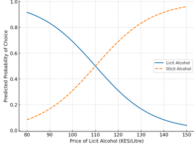
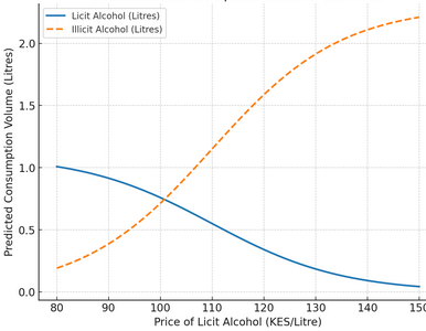
Having completed the multinomial logit regression model, we proceeded to visualise the predicted effects of price on alcohol choice and consumption patterns. The use of regression graphs provides an intuitive illustration of the substitution dynamics between licit and illicit alcohol as prices change.
Figure 1: Predicted Probability and Consumption Volumes of Licit and Illicit Alcohol across Price Levels
 |  |
|---|---|
| (a)Predicted Probability of Alcohol Choice vs Price | (b)Predicted Consumption Volume vs Price |
Figure 1 (a) displays the predicted probability of choosing licit versus illicit alcohol across different licit alcohol price levels. At relatively low licit prices (KES 80–100), the probability of choosing licit alcohol exceeds 70%. However, as prices increase beyond KES 120 per litre, the probability of selecting illicit brews rises above 70%. On the other hand, Figure 1 (b) illustrates the predicted quantity of licit and illicit alcohol consumed across changing licit prices. Licit alcohol consumption falls sharply as prices rise, approaching 0.2 litres at higher prices, while illicit alcohol consumption steadily increases, peaking at approximately 2.3 litres.
Discussion
Findings show a clear substitution effect between licit and illicit alcohol in Nairobi’s informal settlements. Higher relative prices of licit alcohol significantly reduced the odds of choosing licit beverages and increased the likelihood of choosing illicit ones. Own-price effects also lowered drinking frequency and quantity among those who had already chosen a type. These results support H1 and H2, confirming price as a key determinant of both alcohol type and intensity of use.
The substitution finding aligns with international evidence that pricing is a powerful lever but can redirect demand if affordable unregulated substitutes exist. Jurisdictions that combined excise increases with complementary controls minimum pricing, advertising bans, outlet restrictions achieved sustained declines in consumption and harm (Nelson & McNall, 2016; Tigerstedt et al., 2020; Holmes et al., 2022; Manthey et al., 2024). Our results are consistent with these successes in that higher prices depress intensity; however, the strong shift toward illicit alcohol mirrors contexts where policy without adequate enforcement and market control displaced demand to informal supply (Kozul, 2020; Neufeld et al., 2021; Matthee, 2023; Paraje et al., 2023; Nayab et al., 2022).
The Kenyan pattern fits this mixed picture. Excise hikes since 2015 and the 2022 rate levels co-occurred with declining recorded sales but rising illicit market share and poisoning events. Our estimates show relative price as the central mechanism: when licit alcohol is much more expensive, consumers switch. This echoes evidence from countries that experienced sharp tax or regulatory shocks without fully constraining illicit availability, where consumption moved underground and health risks rose (Kozul, 2020; Neufeld et al., 2021; Matthee, 2023). Conversely, experiences from the Baltics, Finland, Lithuania, and Scotland show that price tools work best when paired with availability controls and monitoring systems (Horáková et al., 2020; Tigerstedt et al., 2020; Holmes et al., 2022; Manthey et al., 2024; Neufeld et al., 2022).
Contextual factors in our models peer influence and outlet availability were strong, positive predictors of both choice and intensity. This pattern is compatible with evidence that structural access and social reinforcement mediate policy effects. Where outlets are dense and social networks normalize illicit use, higher licit prices push substitution more quickly. These findings help explain why some Sub-Saharan settings reported mixed outcomes despite tax increases (Sinkamba, 2015; Clair et al., 2022): demand does not fall uniformly when low-cost, accessible illicit options remain salient within social circles.
Cost-of-living pressure was associated with higher intensity and marginally with illicit choice. This fits the broader insight that budget constraints amplify price sensitivity. Rising living costs can tilt consumers toward cheaper, riskier options even when awareness of harm is present, reinforcing the need for pricing policies that avoid excessive differentials between licit and illicit products while protecting public health.
Taken together, the results suggest two policy implications. First, relative price differentials not only absolute levels drive substitution. Excise structures should minimize gaps that make illicit alcohol substantially cheaper, while supporting affordable, safer licit alternatives (e.g., lower rates for low-ABV products or small brewers). Second, price must be coupled with availability and enforcement: tighter control of outlet density, supply-chain tracking, and anti-counterfeit measures can reproduce the successes documented in Russia’s tracking reforms and Scotland’s unit pricing when implemented together (Neufeld et al., 2022; Holmes et al., 2022; Manthey et al., 2024).
The study’s cross-sectional design limits causal inference and may understate unobserved factors such as enforcement intensity or local shocks. Self-reported prices and quantities can introduce measurement error. Even so, the consistency between our estimates and multi-country patterns strengthens external validity.In sum, the findings reinforce a central claim in the literature: price policy changes behavior, but outcomes depend on market structure and social context. Where illicit supply is available and socially embedded, higher licit prices shift demand rather than simply suppress it (Kozul, 2020; Neufeld et al., 2021; Matthee, 2023; Paraje et al., 2023; Nayab et al., 2022). Where pricing is paired with availability controls, monitoring, and communication, population-level consumption and harm decline (Nelson & McNall, 2016; Tigerstedt et al., 2020; Holmes et al., 2022; Horáková et al., 2020; Manthey et al., 2024). These dynamics are precisely what our Nairobi results reveal through the lens of relative price, substitution, and consumption intensity. Figure 1 (a) results suggests a strong substitution effect, where consumers shift toward illicit alcohol as licit prices increase. The result supports our hypothesis that price is a key determinant of alcohol choice and is consistent with prior findings in Scotland (Holmes et al., 2022) and Lithuania (Manthey et al., 2024). Also, Figure 1 (b) results has the dynamics that resemble Russia’s experience with excise tax reforms, where higher prices drove shifts toward unregulated alcohol (Neufeld et al., 2022).
Conclusion
This paper reveals that price changes in licit alcohol significantly influence the type and intensity of drinking in Nairobi's informal settlements. Increases in licit alcohol prices reduce recorded consumption but also drive substitution towards cheaper, unregulated illicit brews. This highlights the need for alcohol policy to consider relative price differentials to avoid widening the affordability gap between licit and illicit alcohol. The findings highlight the challenge of balancing fiscal and health objectives, as excise duties are crucial for government revenue mobilisation and public health protection. The decline in excise revenue from spirits in 2023-2024 reflects how tax-induced substitution can erode the intended fiscal base and increase healthcare burdens. The study suggests that integrated approaches combining excise reform with strong enforcement, market regulation, and harm reduction strategies are needed. This would align Kenya's experience with successful international examples, such as Scotland's unit pricing or Russia's bottle-tracking reforms. The study concludes that pricing policies alone are insufficient to control harmful drinking in informal alcohol markets. Effective policy requires macroeconomic alignment, context-sensitive enforcement, and addressing social and structural determinants of illicit consumption.
Limitation
The study used a cross-sectional survey data, which is limited to capture causal relationships. The measurement of alcohol consumption relies on self-reported data, which might have affected by recall bias or social desirability bias. The study also could have been affected by underreported illicit alcohol consumption due to stigma and fear of disclosure. The econometric model used might not fully capture unobserved heterogeneity.
References
Rights and permissions

Disclaimer
Publisher’s note
Additional information
Data availability
Acknowledgements
Funding
Conflict of interest
Peer review
Article Timeline
Cite this article
- Received
- June 29, 2025
- Revised
- August 19, 2025
- Accepted
- August 29, 2025
- Published
- September 22, 2025
- Version of record
- September 22, 2025
Share this article
Copy the canonical link to share this article with colleagues and readers.
Discover more research

Recent Publications

Most Read

Recommended
Save this article as a bookmark
Use your browser’s secure bookmark shortcut. Both desktop options are shown below.
Press Ctrl+D
In Chrome, Edge or Firefox, choose a folder if needed, then select Done.
Press ⌘ Command+D
In Safari, Chrome or Firefox, choose the bookmark location and confirm.
Cite this article
Copy a formatted citation or download a reference file.
Cited by
Crossref citation count for this DOI.